Inquiry about Kwant boundstate algorithm (unphysical spectra at some sets of parameters)

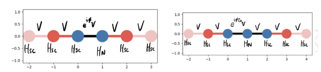
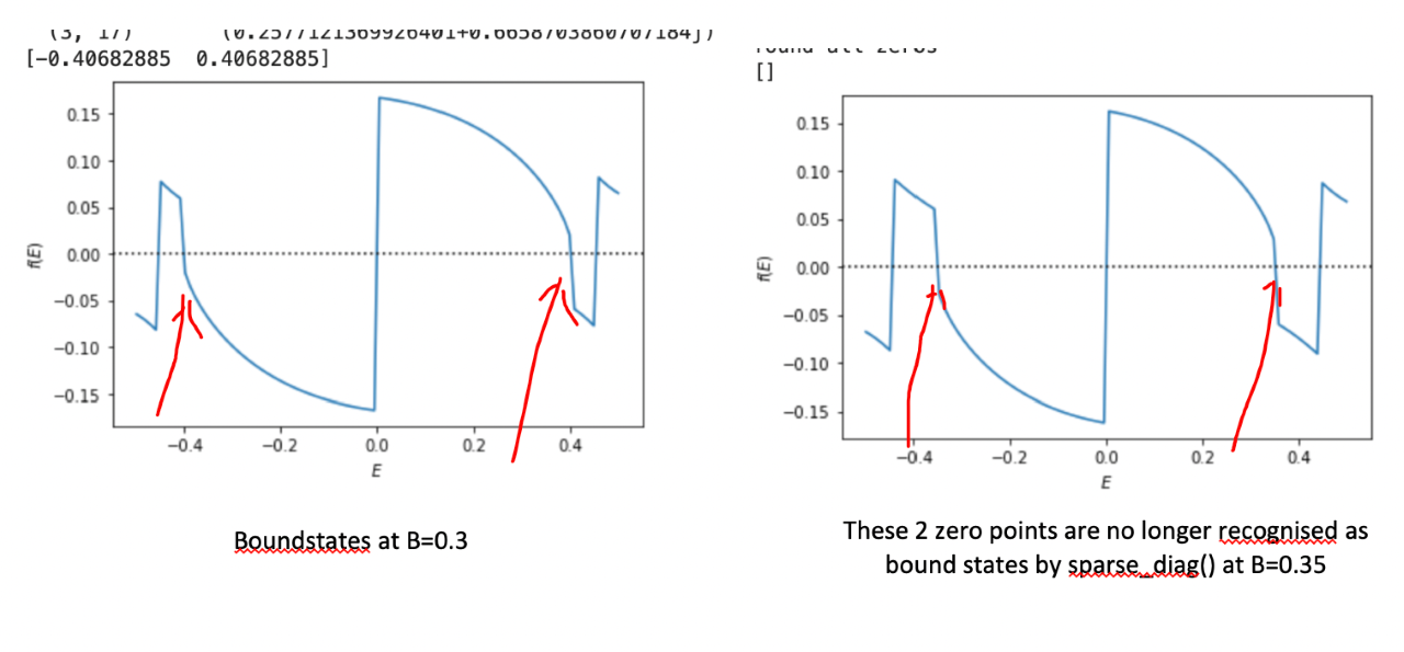
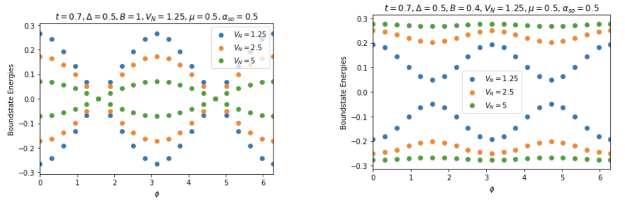
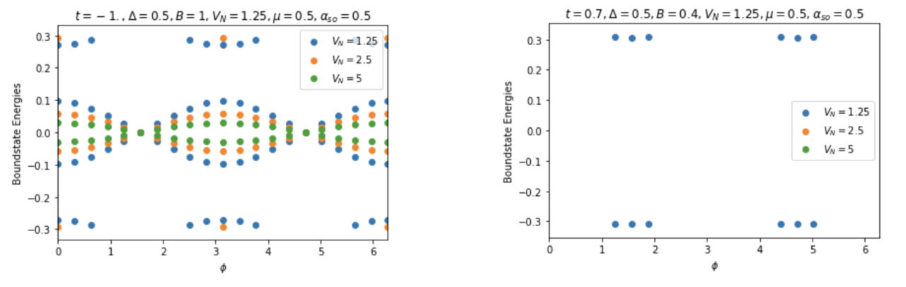
Dear Colleagues, Hi, we are 2 students at Imperial College looking to incorporate your boundstate algorithm (https://scipost.org/submissions/1711.08250v1https://scipost.org/submissions/1711.08250v1/) in the context of a lateral Josephson junction. The code we used was copied and pasted from here: ( https://gitlab.kwant-project.org/jbweston/kwant/-/blob/feature/boundstate/kw...) As an exercise we are trying to reproduce fig. 9 in this paper. Implementing the same parameters, we managed to obtain similar graphs shown below for a value of t=0.7. [cid:d6350847-a84d-413c-966e-9f76a7e16b14] However, we notice that at some values of t, the boundstate algorithm starts yielding non-physical results. Examples include: 1. 1. At t=-1 (which is what we assumed t to be initially from the captions in fig. 7), the algorithm returned energies above the band gap in the JJ in topological regime for some values of phi, the phase difference, and returned true values for some values of phi but not for others in the trivial regime. 2. [cid:ab6b6f7d-c949-4867-a1de-fc904e9d617f] 1. In the B scan for t=-1 boundstates start disappearing from B=0.325 onwards, well before crossing the degeneracy point, and in the topological regime they do not line up with the band edge. 2. [cid:1390ff07-aa3a-4545-ae1b-11b041706548] 1. We also noticed that the algorithm results are dependent on the system setup. To be able to independently replicate fig. 9 my partner and I set up a 2-site (left lead - super - normal - right lead) and 3-site (left lead - super - normal - super - right lead) system respectively to implement the phase from crossing the S-N interface. A schematic of this is shown below. 2. [cid:ccd40751-9e75-4c9f-9dc1-66343648e586] 3. While most standard kwant functionalities seem to recognise the 2 systems are equivalent to each other, we obtained drastically different results from the boundstate algorithm. Examples include a t-scan at B=1 to uncover possible t values where physical ABS spectra could be returned. 4. [cid:d9ca0c7e-5d9f-4546-aadb-091d36aa3542] 5. 2 site 3 site 6. (We checked that the thing causing the drastically different behaviour is the number of sites in the system. We were able to replicate each other's results only by changing the number of sites in the scattering region.) 1. We plotted f(E) in the find_boundstate function for t=-1, B=0.3 (where the algorithm succeeds in detecting the bound state) and B=0.35 (where the algorithm fails to do so), respectively. We noticed that the 2 roots from B=0.3 which are validated to be the true bound states are omitted in B=0.35, not because the validation operator rejects them, but because min_eigenvalue() (or lowest value of sparse_diag()) at these 2 energies indeed returned a value much larger than tol=1e-8 (0.003). We incremented the B field to see when the boundstate to no-boundstate transition occurs and it's at B=0.325 that the min_eigenvalue suddenly shoots up to 1e-4 (for B=0.324 we have 1e-9). We do not understand how this comes to be. 2. [cid:b7e35a85-363c-47d1-b756-52827f73d3f5] 3. The above disappearance of boundstates past B=0.325 is encountered when we set sparse=False too. We would like to know if similar problems with the boundstate algorithm have been encountered before, and if so, what do these signatures tell us is wrong, or does this indeed suggest something is incomplete in the implementation? Finally, we would also like to ask about your specific system setup in Kwant to obtain figure 9, as well as the parameter t that was used, as this was not specified explicitly. Many thanks in advance for answering our query! Sincerely, Chi Zhang & Ryan Tiew Blackett Laboratory Imperial College London

Dear Chi Zhang,
Thank you for your feedback. The implementation that
you have used is due to Joseph Weston and is indeed not
yet completed (which is why it has not been put in the Kwant package so far).
The infrastructure is there, but the algorithm to finds the zeros of f(E) is not yet robust. This is due in part to the fact that Joe did not have a lot of time to invest in this project and in part to the fact that finding such a robust algorithm is beyond a mere implementation and requires a bit of extra research. Indeed, while f(E) is perfectly smooth and any root finder should work, it has occasional jumps that prevent a direct use of these routines. The solution is probably to first detect these jumps but we have not yet tried that and no student is working on the project at the moment. In any case, even if the zeros cannot be found, the results should *not* depend on how you split your system between leads and central part so there might be a bug there as well which we were not aware of, thanks for pointing it out.
I will do some digging to find out the parameters you're looking for and let you know.
Kind regards,
Xavier
________________________________
De : Zhang, Chi

Good afternoon,
Attached in this email is a notebook summarising the investigation we have done so far on the 1D JJ, and the code that we used to create the systems. We were wondering if it would be feasible to have a short meeting online to discuss the algorithm/parameters so that we can progress further with the algorithm.
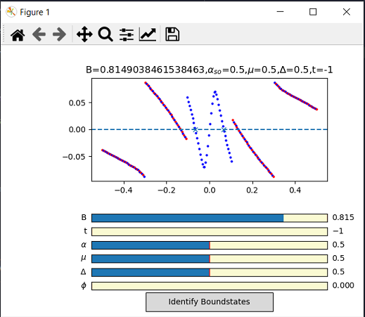
We have also progressed with visual inspections of the root-finding and plotting of f(E) against E. Plots have been color-coded so that lines of a single color represent those with the same wave_functions property in the lead.modes.PropagatingModes. An example of this is shown below, with the B-scan for reference.
[cid:4c5b34e6-f0b2-46fd-9912-0c68ac459421][cid:86af6804-3fcd-4c61-952d-5cff23584e0b][cid:c2739e00-f52d-42c0-a572-b4d6d868cfd3]
Lines that previously appeared continuous seem to have changing propagating mode wavefunctions, and are not accepted as valid solutions. Meanwhile, those that do have the same wavefunctions when E is varied are accepted when there is a root (plotted as crosses on the horizontal axis). The extra states at high B are also seen to be crossings. We also observe different regions and discontinuities. The visual plots seem to be able to identify solutions that are accepted by the algorithm, but we cannot explain why the 2/3-site implementations have different results; these interactive plots have also been included in the notebook.
Regards,
Chi Zhang and Ryan Tiew
________________________________
From: WAINTAL Xavier 200275

Zhang, Chi wrote:
Hi, we are 2 students at Imperial College looking to incorporate your boundstate algorithm (https://scipost.org/submissions/1711.08250v1) in the context of a lateral Josephson junction. (...)
If you guys come up with a module that is more polished than what we have currently please do make it available to the community! Cheers Christoph
participants (4)
-
 Christoph Groth
 -
 Tiew, Hoe R
 -
 WAINTAL Xavier 200275
 -
 Zhang, Chi