Dear Gongwei, Please take a look at the discretizer module introduced in Kwant 1.3 for dealing with tight binging approximations of continuum Hamiltonians. It should save you a lot of work and debugging. As far as the reproducing the results of the reference, I fear it is beyond the scope of this mailing list, and I recommend you to approach the authors directly. Best, Anton On Fri, Sep 8, 2017, 07:35 Gongwei_Hu wrote:

Hello everyone!

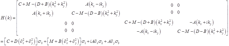
I want to solve a quantum transport question about the quantum spin Hall bar. The Hamiltonian of my system is

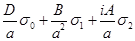
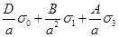
The tight-binding model can be written as follow ( is the lattice constant):

Onsite item: ; Hopping-x item: ; Hopping-y item:

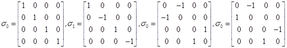
The matrix:

My Question:

(1) The first one is that I am not sure whether the tight-binding model presented above is right for the case of , such as , especially for the hopping –x and –y item.

(2) In order to calculate the density distribution of electron and the conductance, the code presented below cannot exactly match the results in the paper [ https://journals.aps.org/prb/abstract/10.1103/PhysRevB.83.081402]. For example the density of states calculated by Kwant near the edge is much thick compared with the paper results. The conductance also cannot give the same result, such as the conductance is 1.1e^2/h for my result but 2.0e^2/h for the paper at Fermi energy 10meV.

My kwant code is

import math

import numpy

from numpy import *

from matplotlib import pyplot

import kwant

import tinyarray

sigma_0 = tinyarray.array([[1, 0, 0, 0], [0, 1, 0 ,0], [0, 0, 1, 0], [0, 0, 0, 1]])

sigma_1 = tinyarray.array([[0, -1, 0, 0], [-1, 0, 0 ,0], [0, 0, 0, 1], [0, 0, 1, 0]])

sigma_2 = tinyarray.array([[1, 0, 0, 0], [0, -1, 0 ,0], [0, 0, 1, 0], [0, 0, 0, -1]])

sigma_3 = tinyarray.array([[0, -1, 0, 0], [1, 0, 0 ,0], [0, 0, 0, -1], [0, 0, 1, 0]])

def make_system(W_QPC):

L1=70

W1=60

L2=70

W=150

A=364.5

B=-686

C=0

D=-512

M=-10

a=2

b=1

def central_region(pos):

x, y = pos

return -(L1 +W1 + L2)/2 < x < (L1 +W1 + L2)/2 and \

abs(y) < (x <= L1-(L1 +W1 + L2)/2) * abs(0.25 * (2 * W-W_QPC) * (math.sin((x+(L1 +W1 + L2)/2)*math.pi/L1 - math.pi/2) + 1)-W) + (x > L1-(L1 +W1 + L2)/2 and x <= (L1+W1-(L1 +W1 + L2)/2)) * W_QPC/2 + (x > (L1 + W1-(L1 +W1 + L2)/2) and x < (L1+W1+L2-(L1 +W1 + L2)/2)) * abs(0.25 * (2 * W-W_QPC) * (math.sin((x-W1/2)*math.pi/L1 + math.pi/2) + 1)-W)

lat = kwant.lattice.square(a)

sys = kwant.Builder()

sys[lat.shape(central_region, (0, 0))] = (C-4*D/a**2)*sigma_0 + (M-4*B/a**2)*sigma_2

sys[kwant.builder.HoppingKind((b, 0), lat, lat)] = D * sigma_0/a**2+B * sigma_2/a**2+1j * A * sigma_1/a

sys[kwant.builder.HoppingKind((0, b), lat, lat)] = D * sigma_0/a**2+B * sigma_2/a**2+ A * sigma_3/a

sym = kwant.TranslationalSymmetry((-a, 0))

lead = kwant.Builder(sym)

lead[(lat(0, y) for y in range(-int(W/2) + 1, int(W/2)))] = (C-4*D/a**2)*sigma_0 + (M-4*B/a**2)*sigma_2

lead[kwant.builder.HoppingKind((b, 0), lat, lat)] = D * sigma_0/a**2+B * sigma_2/a**2+1j * A * sigma_1/a

lead[kwant.builder.HoppingKind((0, b), lat, lat)] = D * sigma_0/a**2+B * sigma_2/a**2+ A * sigma_3/a

sys.attach_lead(lead)

sys.attach_lead(lead.reversed())

return sys.finalized()

def density(sys, energy):

psi = kwant.wave_function(sys, energy)

for i in range(2):

psi_5 = abs(psi(0)[i]**2)#.sum(axis=0)

#psi_5 = abs(psi(0)[5]**2)

#numpy.savetxt("psi_n.txt",psi_n);

A1, A2 = psi_5[::4], psi_5[1::4]#, psi_n[2::4], psi_n[3::4]

D = A1+A2

numpy.savetxt("D_now.txt",D);

kwant.plotter.map(sys, D)

def plot_conductance(WW_QPC, energy):

# Compute conductance

data = []

for w_QPC in WW_QPC:

sys = make_system(W_QPC=w_QPC)

#sys = sys.finalized()

smatrix = kwant.smatrix(sys, energy)

data.append(smatrix.transmission(1, 0))

numpy.savetxt("WW_QPC.txt",WW_QPC)

numpy.savetxt("data.txt",data)

pyplot.figure()

pyplot.plot(WW_QPC, data)

pyplot.xlabel("W_QPC [nm]")

pyplot.ylabel("conductance [e^2/h]")

pyplot.show()

sys = make_system(W_QPC=50)

kwant.plot(sys)

d = density(sys, energy=10)

plot_conductance(WW_QPC = [50*i+50 for i in range(4)], energy = 10)

#numpy.savetxt("D.txt",d);

#kwant.plotter.map(sys, d)