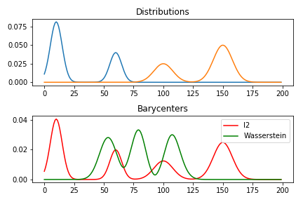
Hello, I am using the following modified code from the tutorial examples/plot_barycenter_1D.py. I have just modified it to compute barycenters between bimodal 1-D distributions. I expected to see the barycenter to also contain only two peaks however it contains 3 which is not very intuitive geometrically speaking . I have attached the resultant figure showing that the barycenter computed has three peaks. Is there a way to intuitively understand why this is happening. The results dont show this if weights computed using \alpha when \alpha = {0,0.1,0.8,0.9,1} Thanks Kowshik import numpy as np import matplotlib.pylab as pl import ot # necessary for 3d plot even if not used from mpl_toolkits.mplot3d import Axes3D # noqa from matplotlib.collections import PolyCollection import os ############################################################################## # Generate data # ------------- #%% parameters n = 200 # nb bins # bin positions x = np.arange(n, dtype=np.float64) # Gaussian distributions a1 = ot.datasets.get_1D_gauss(n, m=10, s=5) # m= mean, s= std a2 = ot.datasets.get_1D_gauss(n, m=60, s=5) # creating matrix A - a bimodal distriution A = a1+0.5*a2 b1 = ot.datasets.get_1D_gauss(n, m=100, s=8) # m= mean, s= std b2 = ot.datasets.get_1D_gauss(n, m=150, s=8) # creating matrix B another bimodal B=0.5*b1+b2 distributions=np.vstack((A,B)).T n_distributions = distributions.shape[1] # loss matrix + normalization M =ot.dist(x.reshape(n,1),x.reshape(n,1),metric= 'sqeuclidean') M /= M.max() ############################################################################## # Plot data # --------- #%% plot the distributions pl.figure(1, figsize=(6.4, 3)) for i in range(n_distributions): pl.plot(x, distributions[:,i]) pl.title('Distributions') pl.tight_layout() ############################################################################## # Barycenter computation # ---------------------- #%% barycenter computation alpha = 0.5 # 0<=alpha<=1 weights = np.array([1 - alpha, alpha]) # l2bary bary_l2 = distributions.dot(weights) # wasserstein reg = 0.001 bary_wass = ot.bregman.barycenter(distributions, M, reg, weights) pl.figure(2) pl.clf() pl.subplot(2, 1, 1) for i in range(n_distributions): pl.plot(x, distributions[:, i]) pl.title('Distributions') pl.subplot(2, 1, 2) pl.plot(x, bary_l2, 'r', label='l2') pl.plot(x, bary_wass, 'g', label='Wasserstein') pl.legend() pl.title('Barycenters') pl.tight_layout()