
Hello everyone, after reading some threads about step response problems in the mailing list i couldnt come up with a proper solution for my problem. I've got the following transfer function: G = Vr/(sT1*(1+sT2)) Vr = 2/15 T1 = 0.2 T2 = 1 For this i like to plot the step response so i made the following script: *---Begin Script* # some imports import numpy as np import matplotlib.pyplot as plt import scipy as sp from scipy import signal # Constants T1 = 0.2 T2 = 1 Vr = float(2)/15 Tsim = 50 # Denumerator N0 = np.array([T1*T2 ,T1 , 0]) # numerator Z0 = Vr # create tfcn sys = sp.signal.lti(Z0, N0) # create the step response t = np.linspace(0, Tsim, 1000) u = np.arange(len(t)) u = np.ones_like(u) yout = sp.signal.lsim2(sys, T=t, U=u)[1] plt.figure(1) plt.plot(t, u, t, yout/yout.max()) plt.grid("on") plt.xlabel("t") plt.ylabel("h(t)") plt.title("Sprungantwort") plt.show() *---End Script* This gives me the following response, which i know is not the rigth one because i made this one already in a lab at university with MATLAB but i don't have MATLAB at home because i prefer to use Numpy+Scipy+Matplotlib. wrong step response Here is the correct response: correct step response After several hours of reading an trying different approaches im kind of frustrated ^^. I would be really thankfull for any help so that i can keep on going the Scipy track. Greetings, William

Le mercredi 23 mai 2012 à 10:01 +0200, otti a écrit :
Hello everyone,
after reading some threads about step response problems in the mailing list i couldnt come up with a proper solution for my problem.
I've got the following transfer function:
G = Vr/(sT1*(1+sT2))
Vr = 2/15 T1 = 0.2 T2 = 1
This transfer function involves an integrator (leading to the slope after the transient) and a first-order low-pass filter (leading to a damped contribution, the transient). IMHO, the step_response.png file is more probably correct than the TA1.jpg file, as there is no second-order term that would possibly lead to the oscillation shown in the latter. Moreover, the action of the integrator for a step response can not lead to a constant steady state. Am I wrong? Looking at the fonts, I believe the step_response.png file comes from matplotlib, and then from your python script. What makes you sure the matlab script is correct? -- Fabrice Silva
Fabrice Silva <silva <at> lma.cnrs-mrs.fr> writes:
This transfer function involves an integrator (leading to the slope after the transient) and a first-order low-pass filter (leading to a damped contribution, the transient).
IMHO, the step_response.png file is more probably correct than the TA1.jpg file, as there is no second-order term that would possibly lead to the oscillation shown in the latter. Moreover, the action of the integrator for a step response can not lead to a constant steady state. Am I wrong?
Looking at the fonts, I believe the step_response.png file comes from matplotlib, and then from your python script. What makes you sure the matlab script is correct?
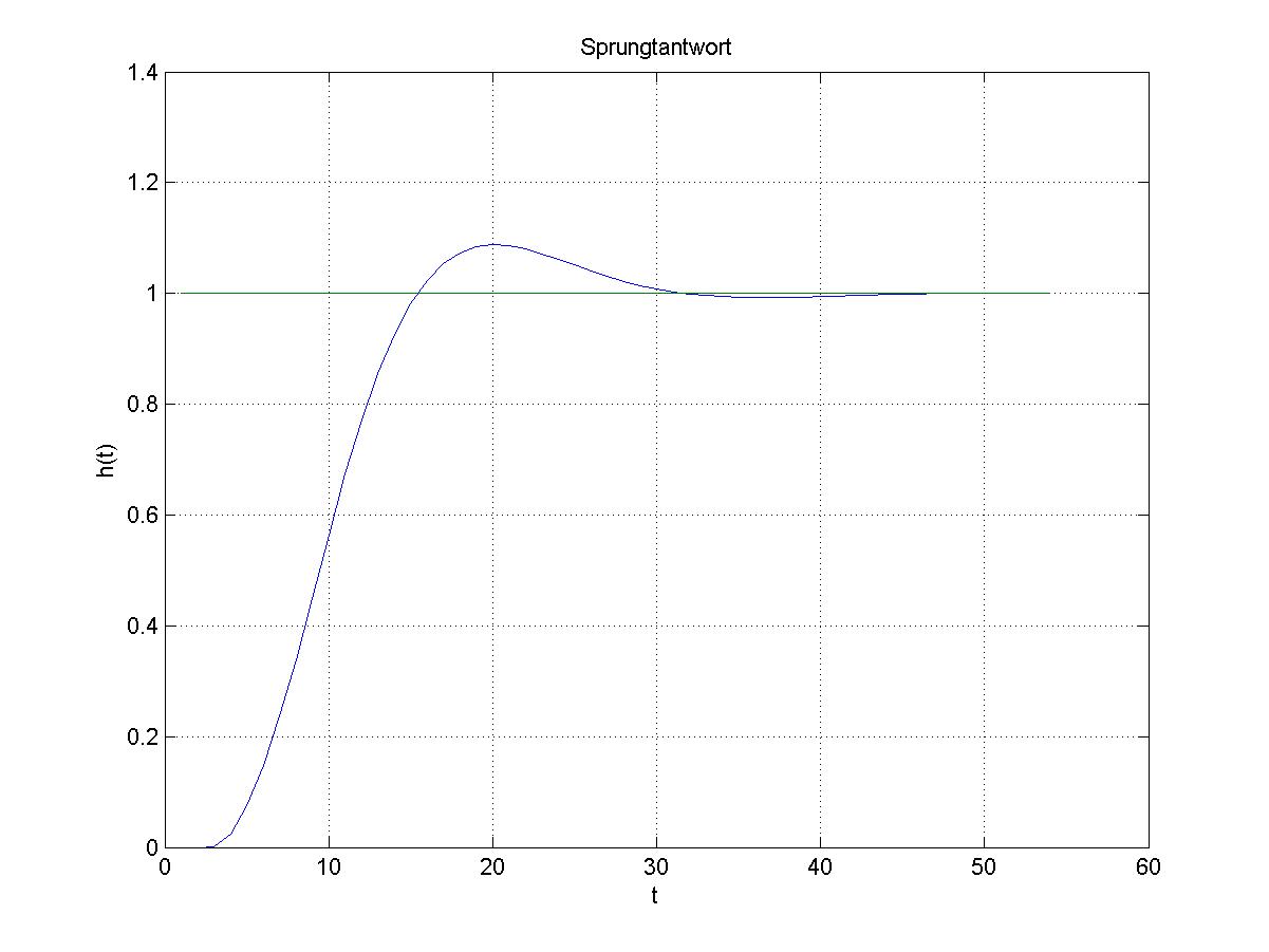
The integrator is used to reduce the overall error of the response so that it reaches the constant steady state 1. The low-pass is used to reduce the overshoot caused by the integrator. If i didn't get it wrong in the control engineering class. Probably have to check the notes again and run thru the MATLAB script again. The response of TA1.jpg was made during a Lab (control engineering) at University and the Prof checked it.
The integrator is used to reduce the overall error of the response so that it reaches the constant steady state 1. The low-pass is used to reduce the overshoot caused by the integrator. If i didn't get it wrong in the control engineering class. Probably have to check the notes again and run thru the MATLAB script again.
The response of TA1.jpg was made during a Lab (control engineering) at University and the Prof checked it.
Are you sure you are not confusing the step response of a transfer function with the step response of a looped system containing an integrator ? Once you close the loop, the global transfer function is not the one you mentionned but H = G/(1+G) for a unity feedback (for example), which exhibits the oscillation and the unity steady state. What you did in your control engineering classes may be the closed-loop system... -- Fabrice Silva
Fabrice Silva <silva <at> lma.cnrs-mrs.fr> writes:
Are you sure you are not confusing the step response of a transfer function with the step response of a looped system containing an integrator ?
Once you close the loop, the global transfer function is not the one you mentionned but H = G/(1+G) for a unity feedback (for example), which exhibits the oscillation and the unity steady state.
Ah thanks alot Fabrice, youre right!! Got things mixed up!
participants (3)
-
 Fabrice Silva
 -
 otti
otti -
William