Elasticity with periodic boundary condition

Dear Robert Cimrman,
I am trying to implement elastic inclusion problem. It is a 2D mesh with an inclusion(and therefore eigenstrain) at mesh centre. I developed my codes(as attached) based on following two previous issues.
https://groups.google.com/forum/#!searchin/sfepy-devel/Ronghai/sfepy-devel/r... https://groups.google.com/forum/#!searchin/sfepy-devel/elastic$20periodic$20boundary$20condition|sort:relevance/sfepy-devel/VpVHXS7Jh0Q/bDNs1JP4x94J
But I have troubles with the boundary conditions. I would like to try two kinds of boundary conditions: (1) Top and bottom boundaries: uniaxial loading(or surface traction). Left and Right boundaries: periodic. I used "dw_tl_surface_traction" but some errors come out. (2) Periodic at all boundaries. I think there must be a easy way for this, but failed to find out in SfePy documentation and mailing list.
Could you please give me some help. Thanks.
Regards Ronghai

Hi Ronghai,
On 02/24/2015 07:29 PM, Ronghai Wu wrote:
Dear Robert Cimrman,
I am trying to implement elastic inclusion problem. It is a 2D mesh with an inclusion(and therefore eigenstrain) at mesh centre. I developed my codes(as attached) based on following two previous issues.
https://groups.google.com/forum/#!searchin/sfepy-devel/Ronghai/sfepy-devel/r... https://groups.google.com/forum/#!searchin/sfepy-devel/elastic$20periodic$20boundary$20condition|sort:relevance/sfepy-devel/VpVHXS7Jh0Q/bDNs1JP4x94J
But I have troubles with the boundary conditions. I would like to try two kinds of boundary conditions: (1) Top and bottom boundaries: uniaxial loading(or surface traction). Left and Right boundaries: periodic. I used "dw_tl_surface_traction" but some errors come out.
Everything is small deformations, right? Then the term to use for tractions is dw_surface_ltr (as in [1]). The term dw_tl_surface_traction is meant for large deformations and is not linear (depends on the actual displacement).
(2) Periodic at all boundaries. I think there must be a easy way for this, but failed to find out in SfePy documentation and mailing list.
What you did works for me (after fixing the term names above). You have the periodic BC on the left and right sides. If you want also top and bottom displacements to be periodic, add an analogous condition.
Also add some Dirichlet BC, so that the matrix is not singular. Anyway, umfpack complains but solves. :) I guess what you need is to have periodic BC left<->right and top<->bottom, and fixed corner nodes, as in [2] (old long syntax...).
Let me know how it goes.
r.
[1] http://sfepy.org/doc-devel/examples/linear_elasticity/linear_elastic_tractio... [2] http://sfepy.org/doc-devel/examples/standalone/homogenized_elasticity/rs_cor...
Hi Robert Cimrman,
Thanks, it helps a lot. But I still have some questions listed below.
Taking the example of a 2D square domain with a circular hole at center,
under tensile traction along x-axis(please see attached
codes"elasticity-periodic BC2").
(1) If the traction stress components are placed in this way?
Material('traction', val=[ [sigma11, sigma12], [sigma21, sigma22] ])
(2) I would like to have tensile traction along x-axis, if the following
codes are correct.
omega = domain.create_region('Omega', 'all')
lef = domain.create_region('Lef', 'vertices in x < %f' % (min_x + eps), 'facet')
rig = domain.create_region('Rig', 'vertices in x > %f' % (max_x - eps), 'facet')
traction_left = Material('traction_left', val=[[1.,0.], [0.,0.]])
traction_right = Material('traction_right', val=[[1.,0.], [0.,0.]])
integral = Integral('i', order=3)
t1 = Term.new('dw_lin_elastic(m.function, v, u )', integral, omega, m=m, v=v, u=u)
t2 = Term.new('dw_lin_prestress(prestress.function, v )',integral, omega, prestress=prestress, v=v)
t3 = Term.new('dw_surface_ltr(traction_left.val, v)', integral, lef, traction_left=traction_left, v=v)
t4 = Term.new('dw_surface_ltr(traction_right.val, v)', integral, rig, traction_right=traction_right, v=v)
fem_eq = Equation('balance', t1 - t2 - t3 - t4 )
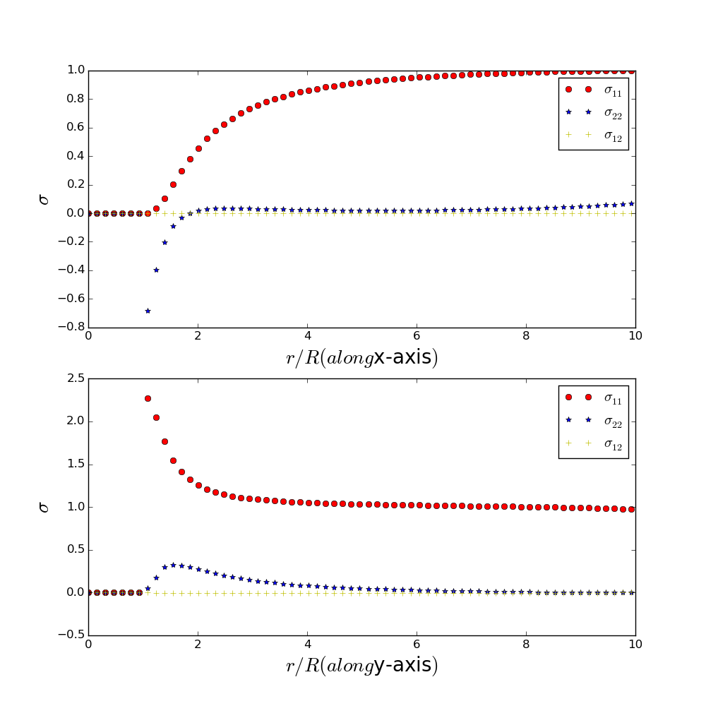
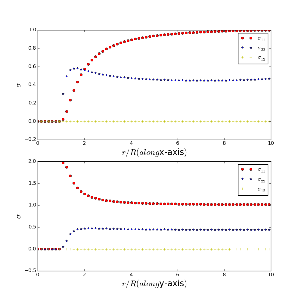
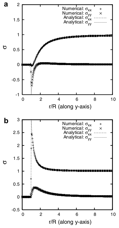
(3) For the boundary condition at top-bottom boundaries, the results are very different between stress-free and periodic BC(please see attached pictures"sfepy stress-free BC" and "sfepy periodic BC"). I also attach the analytical solution for periodic BC case(see "Analytical solution for periodic BC"). However, I found that the sfepy result of stress-free BC agrees well with analytical periodic BC, but sfepy result of periodic BC does not agree with them. This is the situation I do not understand. And I am wondering, do you have other examples with analytical solution which can benchmark the stress-free and periodic BC.
Stress is plotted in this way. A line along x-axis(or y-axis) across the center of hole, plot from the center of hole to boundary, distance(r) is normalized by hole radius(R).
(4) If I would like to run it in parallel. How should I modify the codes?
Regards Ronghai
在 2015年2月26日星期四 UTC+1上午10:54:05,Robert Cimrman写道:
Hi Ronghai,
On 02/24/2015 07:29 PM, Ronghai Wu wrote:
Dear Robert Cimrman,
I am trying to implement elastic inclusion problem. It is a 2D mesh with an inclusion(and therefore eigenstrain) at mesh centre. I developed my codes(as attached) based on following two previous issues.
https://groups.google.com/forum/#!searchin/sfepy-devel/Ronghai/sfepy-devel/r...
But I have troubles with the boundary conditions. I would like to try
two
kinds of boundary conditions: (1) Top and bottom boundaries: uniaxial loading(or surface traction). Left and Right boundaries: periodic. I used "dw_tl_surface_traction" but some errors come out.
Everything is small deformations, right? Then the term to use for tractions is dw_surface_ltr (as in [1]). The term dw_tl_surface_traction is meant for large deformations and is not linear (depends on the actual displacement).
(2) Periodic at all boundaries. I think there must be a easy way for this, but failed to find out in SfePy documentation and mailing list.
What you did works for me (after fixing the term names above). You have the periodic BC on the left and right sides. If you want also top and bottom displacements to be periodic, add an analogous condition.
Also add some Dirichlet BC, so that the matrix is not singular. Anyway, umfpack complains but solves. :) I guess what you need is to have periodic BC left<->right and top<->bottom, and fixed corner nodes, as in [2] (old long syntax...).
Let me know how it goes.
r.
[1]
http://sfepy.org/doc-devel/examples/linear_elasticity/linear_elastic_tractio... [2]
http://sfepy.org/doc-devel/examples/standalone/homogenized_elasticity/rs_cor...
On 03/03/2015 01:16 PM, Ronghai Wu wrote:
Hi Robert Cimrman,
Thanks, it helps a lot. But I still have some questions listed below. Taking the example of a 2D square domain with a circular hole at center, under tensile traction along x-axis(please see attached codes"elasticity-periodic BC2"). (1) If the traction stress components are placed in this way? Material('traction', val=[ [sigma11, sigma12], [sigma21, sigma22] ])
No, it uses the symmetric storage vector: sigma11, sigma22, sigma12. I will update the term docstring.
(2) I would like to have tensile traction along x-axis, if the following codes are correct.
omega = domain.create_region('Omega', 'all')
lef = domain.create_region('Lef', 'vertices in x < %f' % (min_x + eps), 'facet')
rig = domain.create_region('Rig', 'vertices in x > %f' % (max_x - eps), 'facet')
traction_left = Material('traction_left', val=[[1.,0.], [0.,0.]])
traction_right = Material('traction_right', val=[[1.,0.], [0.,0.]])
So this should be:
traction_lef = Material('traction_lef', val=[[1.], [0.], [0.]]) traction_rig = Material('traction_rig', val=[[1.], [0.], [0.]])
integral = Integral('i', order=3)
t1 = Term.new('dw_lin_elastic(m.function, v, u )', integral, omega, m=m, v=v, u=u)
t2 = Term.new('dw_lin_prestress(prestress.function, v )',integral, omega, prestress=prestress, v=v)
t3 = Term.new('dw_surface_ltr(traction_left.val, v)', integral, lef, traction_left=traction_left, v=v)
t4 = Term.new('dw_surface_ltr(traction_right.val, v)', integral, rig, traction_right=traction_right, v=v)
fem_eq = Equation('balance', t1 - t2 - t3 - t4 )
Note here: t3 acts on a boundary, that is completely fixed, so it can be safely removed.
Or, I would use the following minimal BC:
#stress free BC pb.time_update(ebcs=Conditions([fix_u_lef_corner, fix_u_rig_corner]))
#top-bottom periodic BC pb.time_update(ebcs=Conditions([fix_u_lef_corner, fix_u_rig_corner]), epbcs=Conditions([periodic_y]), functions=functions_y)
with:
fix_u_lef_corner = EssentialBC('fix_u_lef_corner', lef_corner, {'u.all' : 0.0}) fix_u_rig_corner = EssentialBC('fix_u_rig_corner', rig_corner, {'u.1' : 0.0})
i.e. no fix_u_lef.
(3) For the boundary condition at top-bottom boundaries, the results are very different between stress-free and periodic BC(please see attached pictures"sfepy stress-free BC" and "sfepy periodic BC"). I also attach the analytical solution for periodic BC case(see "Analytical solution for periodic BC"). However, I found that the sfepy result of stress-free BC agrees well with analytical periodic BC, but sfepy result of periodic BC does not agree with them. This is the situation I do not understand. And I am wondering, do you have other examples with analytical solution which can benchmark the stress-free and periodic BC.
IMHO the results correspond well to the boundary conditions: by imposing the periodic BC on top and bottom, you in fact prevent the narrowing of the domain in the y direction, so sigma_22 has to be positive. Is the analytical result really for the boundary conditions you assume?
Stress is plotted in this way. A line along x-axis(or y-axis) across the center of hole, plot from the center of hole to boundary, distance(r) is normalized by hole radius(R).
BTW. you can get the stress by using the ev_cauchy_stress term, just like the strain... also check the primer for data probes.
(4) If I would like to run it in parallel. How should I modify the codes?
This is work in very slow progress. Not currently possible.
r.
Regards Ronghai
在 2015年2月26日星期四 UTC+1上午10:54:05,Robert Cimrman写道:
Hi Ronghai,
On 02/24/2015 07:29 PM, Ronghai Wu wrote:
Dear Robert Cimrman,
I am trying to implement elastic inclusion problem. It is a 2D mesh with an inclusion(and therefore eigenstrain) at mesh centre. I developed my codes(as attached) based on following two previous issues.
https://groups.google.com/forum/#!searchin/sfepy-devel/Ronghai/sfepy-devel/r...
But I have troubles with the boundary conditions. I would like to try
two
kinds of boundary conditions: (1) Top and bottom boundaries: uniaxial loading(or surface traction). Left and Right boundaries: periodic. I used "dw_tl_surface_traction" but some errors come out.
Everything is small deformations, right? Then the term to use for tractions is dw_surface_ltr (as in [1]). The term dw_tl_surface_traction is meant for large deformations and is not linear (depends on the actual displacement).
(2) Periodic at all boundaries. I think there must be a easy way for this, but failed to find out in SfePy documentation and mailing list.
What you did works for me (after fixing the term names above). You have the periodic BC on the left and right sides. If you want also top and bottom displacements to be periodic, add an analogous condition.
Also add some Dirichlet BC, so that the matrix is not singular. Anyway, umfpack complains but solves. :) I guess what you need is to have periodic BC left<->right and top<->bottom, and fixed corner nodes, as in [2] (old long syntax...).
Let me know how it goes.
r.
[1]
http://sfepy.org/doc-devel/examples/linear_elasticity/linear_elastic_tractio... [2]
http://sfepy.org/doc-devel/examples/standalone/homogenized_elasticity/rs_cor...
在 2015年3月3日星期二 UTC+1下午11:35:05,Robert Cimrman写道:
On 03/03/2015 01:16 PM, Ronghai Wu wrote:
Hi Robert Cimrman,
Thanks, it helps a lot. But I still have some questions listed below. Taking the example of a 2D square domain with a circular hole at center, under tensile traction along x-axis(please see attached codes"elasticity-periodic BC2"). (1) If the traction stress components are placed in this way? Material('traction', val=[ [sigma11, sigma12], [sigma21, sigma22] ])
No, it uses the symmetric storage vector: sigma11, sigma22, sigma12. I will update the term docstring.
(2) I would like to have tensile traction along x-axis, if the following codes are correct.
omega = domain.create_region('Omega', 'all')
lef = domain.create_region('Lef', 'vertices in x < %f' % (min_x + eps), 'facet')
rig = domain.create_region('Rig', 'vertices in x > %f' % (max_x - eps), 'facet')
traction_left = Material('traction_left', val=[[1.,0.], [0.,0.]])
traction_right = Material('traction_right', val=[[1.,0.], [0.,0.]])
So this should be:
traction_lef = Material('traction_lef', val=[[1.], [0.], [0.]]) traction_rig = Material('traction_rig', val=[[1.], [0.], [0.]])
integral = Integral('i', order=3)
t1 = Term.new('dw_lin_elastic(m.function, v, u )', integral, omega, m=m, v=v, u=u)
t2 = Term.new('dw_lin_prestress(prestress.function, v )',integral,
omega,
prestress=prestress, v=v)
t3 = Term.new('dw_surface_ltr(traction_left.val, v)', integral, lef, traction_left=traction_left, v=v)
t4 = Term.new('dw_surface_ltr(traction_right.val, v)', integral, rig, traction_right=traction_right, v=v)
fem_eq = Equation('balance', t1 - t2 - t3 - t4 )
Note here: t3 acts on a boundary, that is completely fixed, so it can be safely removed.
Or, I would use the following minimal BC:
#stress free BC pb.time_update(ebcs=Conditions([fix_u_lef_corner, fix_u_rig_corner]))
#top-bottom periodic BC pb.time_update(ebcs=Conditions([fix_u_lef_corner, fix_u_rig_corner]), epbcs=Conditions([periodic_y]), functions=functions_y)
with:
fix_u_lef_corner = EssentialBC('fix_u_lef_corner', lef_corner, {'u.all' : 0.0}) fix_u_rig_corner = EssentialBC('fix_u_rig_corner', rig_corner, {'u.1' : 0.0})
i.e. no fix_u_lef.
Thanks, I corrected the codes accordingly.
(3) For the boundary condition at top-bottom boundaries, the results are very different between stress-free and periodic BC(please see attached pictures"sfepy stress-free BC" and "sfepy periodic BC"). I also attach
the
analytical solution for periodic BC case(see "Analytical solution for periodic BC"). However, I found that the sfepy result of stress-free BC agrees well with analytical periodic BC, but sfepy result of periodic BC does not agree with them. This is the situation I do not understand. And I am wondering, do you have other examples with analytical solution which can benchmark the stress-free and periodic BC.
IMHO the results correspond well to the boundary conditions: by imposing the periodic BC on top and bottom, you in fact prevent the narrowing of the domain in the y direction, so sigma_22 has to be positive. Is the analytical result really for the boundary conditions you assume?
You are right. I got the analytical from a paper which says the boundary condition is periodic. But I checked more papers and found out the actual boundary condition is stress free.
Stress is plotted in this way. A line along x-axis(or y-axis) across the center of hole, plot from the center of hole to boundary, distance(r) is normalized by hole radius(R).
BTW. you can get the stress by using the ev_cauchy_stress term, just like the strain... also check the primer for data probes.
I tried to do this, but got error which I cannot fix (please run "elasticity-periodicBC3.py"). Additionally, I have some questions regarding the strain and stress calculated by pb.evalate(please see "questions about strain and stress.pdf").
Regards, Ronghai
On 03/05/2015 05:01 PM, Ronghai Wu wrote:
在 2015年3月3日星期二 UTC+1下午11:35:05,Robert Cimrman写道:
<snip>
Stress is plotted in this way. A line along x-axis(or y-axis) across the center of hole, plot from the center of hole to boundary, distance(r) is normalized by hole radius(R).
BTW. you can get the stress by using the ev_cauchy_stress term, just like the strain... also check the primer for data probes.
I tried to do this, but got error which I cannot fix (please run "elasticity-periodicBC3.py"). Additionally, I have some questions regarding the strain and stress calculated by pb.evalate(please see "questions about strain and stress.pdf").
You just need to use the probing code from examples/linear_elasticity/its2D_interactive.py, because your script is also interactive. Attached is the fixed script (+ some additional small fixes).
As for the questions, the strain and stress coming from ev_cauchy_*() terms are without the prestrain. You need to subtract that yourself.
r.
Thanks a lot. My complete problem is actually a dynamic problem, at every time-step run sfepy as stress-strain solver. However, when the mesh is large such as 513*513, sfepy runs slowly, especially during solving equlibrium equation from iter 0 to iter 1. The solving process takes roughly 1 min/time-step. I am wondering is there any good idea to improve the running speed?
在 2015年3月5日星期四 UTC+1下午5:37:00,Robert Cimrman写道:
On 03/05/2015 05:01 PM, Ronghai Wu wrote:
在 2015年3月3日星期二 UTC+1下午11:35:05,Robert Cimrman写道:
<snip>
Stress is plotted in this way. A line along x-axis(or y-axis) across the center of hole, plot from the center of hole to boundary, distance(r) is normalized by hole radius(R).
BTW. you can get the stress by using the ev_cauchy_stress term, just like the strain... also check the primer for data probes.
I tried to do this, but got error which I cannot fix (please run "elasticity-periodicBC3.py"). Additionally, I have some questions regarding the strain and stress calculated by pb.evalate(please see "questions about strain and stress.pdf").
You just need to use the probing code from examples/linear_elasticity/its2D_interactive.py, because your script is also interactive. Attached is the fixed script (+ some additional small fixes).
As for the questions, the strain and stress coming from ev_cauchy_*() terms are without the prestrain. You need to subtract that yourself.
r.
On 03/09/2015 10:22 PM, Ronghai Wu wrote:
Thanks a lot. My complete problem is actually a dynamic problem, at every time-step run sfepy as stress-strain solver. However, when the mesh is large such as 513*513, sfepy runs slowly, especially during solving equlibrium equation from iter 0 to iter 1. The solving process takes roughly 1 min/time-step. I am wondering is there any good idea to improve the running speed?
The problem is linear, right? Then try setting the 'is_linear' option of the Newton solver [1] to True. Then the matrix is assembled only once, and, in case you use the ls.scipy_direct solver, also prefactorized. So the first time step will be slow, but the other steps fast. If the problem is too big for the direct solver, try using and iterative solver instead. I have a good experience with the ones in petsc [2].
r.
[1] http://sfepy.org/doc-devel/src/sfepy/solvers/nls.html?highlight=is_linear [2] http://sfepy.org/doc-devel/src/sfepy/solvers/ls.html#sfepy.solvers.ls.PETScK...
Yes, it is linear elasticity problem.
If using linear Newton solver, do you exactly mean ?
ls = ScipyDirect({})
nls_status = IndexedStruct()
nls = Newton({'problem' : 'linear'}, lin_solver=ls, status=nls_status)
pb = Problem('elasticity', equations=eqs, nls=nls, ls=ls)
and if using PETScKrylovSolver, do you exactly mean ?
ls = PETScKrylovSolver({})
pb = Problem('elasticity', equations=eqs, ls=ls)
Another question in the ''Interactive Example: Linear Elasticity'' : In [23]: bc_fun = Function(’shift_u_fun’, shift_u_fun, extra_args={’shift’ : 0.01}) In [24]: shift_u = EssentialBC(’shift_u’, gamma2, {’u.0’ : bc_fun}) is this shift a necessity to get correct result? I mean without this, if the result will be ridiculous or basically right? Thanks
在 2015年3月11日星期三 UTC+1下午4:14:30,Robert Cimrman写道:
On 03/09/2015 10:22 PM, Ronghai Wu wrote:
Thanks a lot. My complete problem is actually a dynamic problem, at every time-step run sfepy as stress-strain solver. However, when the mesh is large such as 513*513, sfepy runs slowly, especially during solving equlibrium equation from iter 0 to iter 1. The solving process takes roughly 1 min/time-step. I am wondering is there any good idea to improve the running speed?
The problem is linear, right? Then try setting the 'is_linear' option of the Newton solver [1] to True. Then the matrix is assembled only once, and, in case you use the ls.scipy_direct solver, also prefactorized. So the first time step will be slow, but the other steps fast. If the problem is too big for the direct solver, try using and iterative solver instead. I have a good experience with the ones in petsc [2].
r.
[1] http://sfepy.org/doc-devel/src/sfepy/solvers/nls.html?highlight=is_linear [2]
http://sfepy.org/doc-devel/src/sfepy/solvers/ls.html#sfepy.solvers.ls.PETScK... http://www.google.com/url?q=http%3A%2F%2Fsfepy.org%2Fdoc-devel%2Fsrc%2Fsfepy%2Fsolvers%2Fls.html%23sfepy.solvers.ls.PETScKrylovSolver&sa=D&sntz=1&usg=AFQjCNGLXWR-zmz9fJJoYchqeeLIrxlbpw
On 03/11/2015 08:02 PM, Ronghai Wu wrote:
Yes, it is linear elasticity problem. If using linear Newton solver, do you exactly mean ? ls = ScipyDirect({}) nls_status = IndexedStruct() nls = Newton({'problem' : 'linear'}, lin_solver=ls, status=nls_status) pb = Problem('elasticity', equations=eqs, nls=nls, ls=ls)
Yes, sorry, I forgot your script is interactive. In SfePy prior to 2015.1 the option is {'problem' : 'linear'}. In 2015.1 it reads {'is_linear' : True}, as 'problem' was ambiguous.
and if using PETScKrylovSolver, do you exactly mean ? ls = PETScKrylovSolver({})
Essentially, yes. The above uses the default solver, preconditioner, tolerances and other options. You may need to experiment with those. Try, for example:
ls = PETScKrylovSolver({ 'method' : 'cg', 'precond' : 'icc' 'eps_r' : 1e-8, 'i_max' : 100, })
and use this as in your snippet above instead of ScipyDirect.
Another question in the ''Interactive Example: Linear Elasticity'' : In [23]: bc_fun = Function(’shift_u_fun’, shift_u_fun, extra_args={’shift’ : 0.01}) In [24]: shift_u = EssentialBC(’shift_u’, gamma2, {’u.0’ : bc_fun}) is this shift a necessity to get correct result? I mean without this, if the result will be ridiculous or basically right? Thanks
Here, the shift is the amplitude of the imposed Dirichlet conditions on gamma2. It serves as an example of how to pass extra arguments to the ebc functions. If you set shift to zero, it would be equivalent to set {'u.0' : 0.0} on the gamma2 boundary. Did I answer your question?
r.
I wrote my codes in sfepy-2014.4, but recently I upgraded to sfepy-2015.1. If every other things are the same except for solvers, I got some cases work and some do not. Do you have any idea about the reason? (1) If I keep the problem as nonlinear, it works(original code) ls = ScipyDirect({'presolve':True}) nls_status = IndexedStruct() nls = Newton({'problem' : 'nonlinear'}, lin_solver=ls, status=nls_status) pb = Problem('elasticity', equations=eqs, nls=nls, ls=ls) ############################################################# sfepy: nls: iter: 0, residual: 2.785678e+02 (rel: 1.000000e+00) sfepy: rezidual: 0.46 [s] sfepy: solve: 57.95 [s] sfepy: matrix: 0.67 [s] sfepy: nls: iter: 1, residual: 2.625559e-11 (rel: 9.425207e-14)
(2) if I change to linear, it does not work. ls = ScipyDirect({'presolve':True}) nls_status = IndexedStruct() nls = Newton({'is_linear' : True}, lin_solver=ls, status=nls_status) pb = Problem('elasticity', equations=eqs, nls=nls, ls=ls) ################################################# sfepy: nls: iter: 0, residual: 2.785678e+02 (rel: 1.000000e+00) virtual201503/local/lib/python2.7/site-packages/scipy/sparse/linalg/dsolve/linsolve.py:145: MatrixRankWarning: Matrix is exactly singular warn("Matrix is exactly singular", MatrixRankWarning) sfepy: rezidual: 0.47 [s] sfepy: solve: 19.58 [s] sfepy: matrix: 0.00 [s] sfepy: linesearch: iter 1, (nan < 2.78565e+02) (new ls: 1.000000e-01) sfepy: linesearch: iter 1, (nan < 2.78565e+02) (new ls: 1.000000e-02) sfepy: linesearch: iter 1, (nan < 2.78565e+02) (new ls: 1.000000e-03) sfepy: linesearch: iter 1, (nan < 2.78565e+02) (new ls: 1.000000e-04) sfepy: linesearch: iter 1, (nan < 2.78565e+02) (new ls: 1.000000e-05) sfepy: linesearch: iter 1, (nan < 2.78565e+02) (new ls: 1.000000e-06) sfepy: linesearch: iter 1, (nan < 2.78565e+02) (new ls: 1.000000e-07) sfepy: linesearch failed, continuing anyway sfepy: nls: iter: 1, residual: nan (rel: nan)
(3)
ls = PETScKrylovSolver({'method' : 'cg', 'precond' : 'icc', 'eps_r' : 1e-8, 'i_max' : 100}) nls_status = IndexedStruct() nls = Newton({'is_linear' : True}, lin_solver=ls, status=nls_status) pb = Problem('elasticity', equations=eqs, nls=nls, ls=ls) ####################################################### sfepy: nls: iter: 0, residual: 2.785678e+02 (rel: 1.000000e+00) sfepy: cg(icc) convergence: -10 (DIVERGED_INDEFINITE_MAT) sfepy: rezidual: 0.47 [s] sfepy: solve: 0.26 [s] sfepy: matrix: 0.00 [s] sfepy: warning: linear system solution precision is lower sfepy: then the value set in solver options! (err = 2.785678e+02 < 1.000000e-10) sfepy: linesearch: iter 1, (2.78568e+02 < 2.78565e+02) (new ls: 1.000000e-01) sfepy: linesearch: iter 1, (2.78568e+02 < 2.78565e+02) (new ls: 1.000000e-02) sfepy: linesearch: iter 1, (2.78568e+02 < 2.78565e+02) (new ls: 1.000000e-03) sfepy: linesearch: iter 1, (2.78568e+02 < 2.78565e+02) (new ls: 1.000000e-04) sfepy: linesearch: iter 1, (2.78568e+02 < 2.78565e+02) (new ls: 1.000000e-05) sfepy: linesearch: iter 1, (2.78568e+02 < 2.78565e+02) (new ls: 1.000000e-06) sfepy: linesearch: iter 1, (2.78568e+02 < 2.78565e+02) (new ls: 1.000000e-07) sfepy: linesearch failed, continuing anyway sfepy: nls: iter: 1, residual: 2.785678e+02 (rel: 1.000000e+00) sfepy: cg(icc) convergence: -10 (DIVERGED_INDEFINITE_MAT) sfepy: rezidual: 0.29 [s] sfepy: solve: 0.26 [s] sfepy: matrix: 0.00 [s] sfepy: warning: linear system solution precision is lower sfepy: then the value set in solver options! (err = 2.785678e+02 < 1.000000e-10) sfepy: linesearch: iter 2, (2.78568e+02 < 2.78565e+02) (new ls: 1.000000e-01) sfepy: linesearch: iter 2, (2.78568e+02 < 2.78565e+02) (new ls: 1.000000e-02) sfepy: linesearch: iter 2, (2.78568e+02 < 2.78565e+02) (new ls: 1.000000e-03) sfepy: linesearch: iter 2, (2.78568e+02 < 2.78565e+02) (new ls: 1.000000e-04) sfepy: linesearch: iter 2, (2.78568e+02 < 2.78565e+02) (new ls: 1.000000e-05) sfepy: linesearch: iter 2, (2.78568e+02 < 2.78565e+02) (new ls: 1.000000e-06) sfepy: linesearch: iter 2, (2.78568e+02 < 2.78565e+02) (new ls: 1.000000e-07) sfepy: linesearch failed, continuing anyway sfepy: nls: iter: 2, residual: 2.785678e+02 (rel: 1.000000e+00) sfepy: equation "tmp":
在 2015年3月12日星期四 UTC+1下午2:50:25,Robert Cimrman写道:
On 03/11/2015 08:02 PM, Ronghai Wu wrote:
Yes, it is linear elasticity problem. If using linear Newton solver, do you exactly mean ? ls = ScipyDirect({}) nls_status = IndexedStruct() nls = Newton({'problem' : 'linear'}, lin_solver=ls, status=nls_status) pb = Problem('elasticity', equations=eqs, nls=nls, ls=ls)
Yes, sorry, I forgot your script is interactive. In SfePy prior to 2015.1 the option is {'problem' : 'linear'}. In 2015.1 it reads {'is_linear' : True}, as 'problem' was ambiguous.
and if using PETScKrylovSolver, do you exactly mean ? ls = PETScKrylovSolver({})
Essentially, yes. The above uses the default solver, preconditioner, tolerances and other options. You may need to experiment with those. Try, for example:
ls = PETScKrylovSolver({ 'method' : 'cg', 'precond' : 'icc' 'eps_r' : 1e-8, 'i_max' : 100, })
and use this as in your snippet above instead of ScipyDirect.
Another question in the ''Interactive Example: Linear Elasticity'' : In [23]: bc_fun = Function(’shift_u_fun’, shift_u_fun, extra_args={’shift’ : 0.01}) In [24]: shift_u = EssentialBC(’shift_u’, gamma2, {’u.0’ : bc_fun}) is this shift a necessity to get correct result? I mean without this, if the result will be ridiculous or basically right? Thanks
Here, the shift is the amplitude of the imposed Dirichlet conditions on gamma2. It serves as an example of how to pass extra arguments to the ebc functions. If you set shift to zero, it would be equivalent to set {'u.0' : 0.0} on the gamma2 boundary. Did I answer your question?
r.
The linear option works in connection with time-stepping solvers. I have found recently, that the time stepping solvers do not play well in interactive building of the problem. The fix should be available soon.
The singular matrix warning is caused by the fact, that in the linear case the non-linear solver assumes that the matrix is already assembled (which is the case, if called from the time-stepping solvers in sfepy). In your script, try calling the following before solving the problem:
# pb = Problem('elasticity', equations=eqs, nls=nls, ls=ls) from sfepy.solvers.ts_solvers import prepare_matrix prepare_matrix(pb, pb.create_state())
r.
On 03/12/2015 06:01 PM, Ronghai Wu wrote:
I wrote my codes in sfepy-2014.4, but recently I upgraded to sfepy-2015.1. If every other things are the same except for solvers, I got some cases work and some do not. Do you have any idea about the reason? (1) If I keep the problem as nonlinear, it works(original code) ls = ScipyDirect({'presolve':True}) nls_status = IndexedStruct() nls = Newton({'problem' : 'nonlinear'}, lin_solver=ls, status=nls_status) pb = Problem('elasticity', equations=eqs, nls=nls, ls=ls) ############################################################# sfepy: nls: iter: 0, residual: 2.785678e+02 (rel: 1.000000e+00) sfepy: rezidual: 0.46 [s] sfepy: solve: 57.95 [s] sfepy: matrix: 0.67 [s] sfepy: nls: iter: 1, residual: 2.625559e-11 (rel: 9.425207e-14)
(2) if I change to linear, it does not work. ls = ScipyDirect({'presolve':True}) nls_status = IndexedStruct() nls = Newton({'is_linear' : True}, lin_solver=ls, status=nls_status) pb = Problem('elasticity', equations=eqs, nls=nls, ls=ls) ################################################# sfepy: nls: iter: 0, residual: 2.785678e+02 (rel: 1.000000e+00) virtual201503/local/lib/python2.7/site-packages/scipy/sparse/linalg/dsolve/linsolve.py:145: MatrixRankWarning: Matrix is exactly singular warn("Matrix is exactly singular", MatrixRankWarning) sfepy: rezidual: 0.47 [s] sfepy: solve: 19.58 [s] sfepy: matrix: 0.00 [s] sfepy: linesearch: iter 1, (nan < 2.78565e+02) (new ls: 1.000000e-01) sfepy: linesearch: iter 1, (nan < 2.78565e+02) (new ls: 1.000000e-02) sfepy: linesearch: iter 1, (nan < 2.78565e+02) (new ls: 1.000000e-03) sfepy: linesearch: iter 1, (nan < 2.78565e+02) (new ls: 1.000000e-04) sfepy: linesearch: iter 1, (nan < 2.78565e+02) (new ls: 1.000000e-05) sfepy: linesearch: iter 1, (nan < 2.78565e+02) (new ls: 1.000000e-06) sfepy: linesearch: iter 1, (nan < 2.78565e+02) (new ls: 1.000000e-07) sfepy: linesearch failed, continuing anyway sfepy: nls: iter: 1, residual: nan (rel: nan)
(3)
ls = PETScKrylovSolver({'method' : 'cg', 'precond' : 'icc', 'eps_r' : 1e-8, 'i_max' : 100}) nls_status = IndexedStruct() nls = Newton({'is_linear' : True}, lin_solver=ls, status=nls_status) pb = Problem('elasticity', equations=eqs, nls=nls, ls=ls) ####################################################### sfepy: nls: iter: 0, residual: 2.785678e+02 (rel: 1.000000e+00) sfepy: cg(icc) convergence: -10 (DIVERGED_INDEFINITE_MAT) sfepy: rezidual: 0.47 [s] sfepy: solve: 0.26 [s] sfepy: matrix: 0.00 [s] sfepy: warning: linear system solution precision is lower sfepy: then the value set in solver options! (err = 2.785678e+02 < 1.000000e-10) sfepy: linesearch: iter 1, (2.78568e+02 < 2.78565e+02) (new ls: 1.000000e-01) sfepy: linesearch: iter 1, (2.78568e+02 < 2.78565e+02) (new ls: 1.000000e-02) sfepy: linesearch: iter 1, (2.78568e+02 < 2.78565e+02) (new ls: 1.000000e-03) sfepy: linesearch: iter 1, (2.78568e+02 < 2.78565e+02) (new ls: 1.000000e-04) sfepy: linesearch: iter 1, (2.78568e+02 < 2.78565e+02) (new ls: 1.000000e-05) sfepy: linesearch: iter 1, (2.78568e+02 < 2.78565e+02) (new ls: 1.000000e-06) sfepy: linesearch: iter 1, (2.78568e+02 < 2.78565e+02) (new ls: 1.000000e-07) sfepy: linesearch failed, continuing anyway sfepy: nls: iter: 1, residual: 2.785678e+02 (rel: 1.000000e+00) sfepy: cg(icc) convergence: -10 (DIVERGED_INDEFINITE_MAT) sfepy: rezidual: 0.29 [s] sfepy: solve: 0.26 [s] sfepy: matrix: 0.00 [s] sfepy: warning: linear system solution precision is lower sfepy: then the value set in solver options! (err = 2.785678e+02 < 1.000000e-10) sfepy: linesearch: iter 2, (2.78568e+02 < 2.78565e+02) (new ls: 1.000000e-01) sfepy: linesearch: iter 2, (2.78568e+02 < 2.78565e+02) (new ls: 1.000000e-02) sfepy: linesearch: iter 2, (2.78568e+02 < 2.78565e+02) (new ls: 1.000000e-03) sfepy: linesearch: iter 2, (2.78568e+02 < 2.78565e+02) (new ls: 1.000000e-04) sfepy: linesearch: iter 2, (2.78568e+02 < 2.78565e+02) (new ls: 1.000000e-05) sfepy: linesearch: iter 2, (2.78568e+02 < 2.78565e+02) (new ls: 1.000000e-06) sfepy: linesearch: iter 2, (2.78568e+02 < 2.78565e+02) (new ls: 1.000000e-07) sfepy: linesearch failed, continuing anyway sfepy: nls: iter: 2, residual: 2.785678e+02 (rel: 1.000000e+00) sfepy: equation "tmp":
在 2015年3月12日星期四 UTC+1下午2:50:25,Robert Cimrman写道:
On 03/11/2015 08:02 PM, Ronghai Wu wrote:
Yes, it is linear elasticity problem. If using linear Newton solver, do you exactly mean ? ls = ScipyDirect({}) nls_status = IndexedStruct() nls = Newton({'problem' : 'linear'}, lin_solver=ls, status=nls_status) pb = Problem('elasticity', equations=eqs, nls=nls, ls=ls)
Yes, sorry, I forgot your script is interactive. In SfePy prior to 2015.1 the option is {'problem' : 'linear'}. In 2015.1 it reads {'is_linear' : True}, as 'problem' was ambiguous.
and if using PETScKrylovSolver, do you exactly mean ? ls = PETScKrylovSolver({})
Essentially, yes. The above uses the default solver, preconditioner, tolerances and other options. You may need to experiment with those. Try, for example:
ls = PETScKrylovSolver({ 'method' : 'cg', 'precond' : 'icc' 'eps_r' : 1e-8, 'i_max' : 100, })
and use this as in your snippet above instead of ScipyDirect.
Another question in the ''Interactive Example: Linear Elasticity'' : In [23]: bc_fun = Function(’shift_u_fun’, shift_u_fun, extra_args={’shift’ : 0.01}) In [24]: shift_u = EssentialBC(’shift_u’, gamma2, {’u.0’ : bc_fun}) is this shift a necessity to get correct result? I mean without this, if the result will be ridiculous or basically right? Thanks
Here, the shift is the amplitude of the imposed Dirichlet conditions on gamma2. It serves as an example of how to pass extra arguments to the ebc functions. If you set shift to zero, it would be equivalent to set {'u.0' : 0.0} on the gamma2 boundary. Did I answer your question?
r.
Thanks, after adding the code before solving, it works. I do not exactly understand what you mean by "time-stepping solvers". This problem exists only in sfepy2015.1 or also in sfepy-2014.4? Do you mean a interactive building problem with codes like "pb.time_update, pb.update_materials" does not not work well currently? I am worrying about the influence of this "time-stepping solvers". Where can I find the fix? also in sfepy-devel?
在 2015年3月13日星期五 UTC+1下午1:42:26,Robert Cimrman写道:
The linear option works in connection with time-stepping solvers. I have found recently, that the time stepping solvers do not play well in interactive building of the problem. The fix should be available soon.
The singular matrix warning is caused by the fact, that in the linear case the non-linear solver assumes that the matrix is already assembled (which is the case, if called from the time-stepping solvers in sfepy). In your script, try calling the following before solving the problem:
# pb = Problem('elasticity', equations=eqs, nls=nls, ls=ls) from sfepy.solvers.ts_solvers import prepare_matrix prepare_matrix(pb, pb.create_state())
r.
On 03/12/2015 06:01 PM, Ronghai Wu wrote:
I wrote my codes in sfepy-2014.4, but recently I upgraded to sfepy-2015.1. If every other things are the same except for solvers, I got some cases work and some do not. Do you have any idea about the reason? (1) If I keep the problem as nonlinear, it works(original code) ls = ScipyDirect({'presolve':True}) nls_status = IndexedStruct() nls = Newton({'problem' : 'nonlinear'}, lin_solver=ls, status=nls_status) pb = Problem('elasticity', equations=eqs, nls=nls, ls=ls) ############################################################# sfepy: nls: iter: 0, residual: 2.785678e+02 (rel: 1.000000e+00) sfepy: rezidual: 0.46 [s] sfepy: solve: 57.95 [s] sfepy: matrix: 0.67 [s] sfepy: nls: iter: 1, residual: 2.625559e-11 (rel: 9.425207e-14)
(2) if I change to linear, it does not work. ls = ScipyDirect({'presolve':True}) nls_status = IndexedStruct() nls = Newton({'is_linear' : True}, lin_solver=ls, status=nls_status) pb = Problem('elasticity', equations=eqs, nls=nls, ls=ls) ################################################# sfepy: nls: iter: 0, residual: 2.785678e+02 (rel: 1.000000e+00)
virtual201503/local/lib/python2.7/site-packages/scipy/sparse/linalg/dsolve/linsolve.py:145: MatrixRankWarning: Matrix is exactly singular
warn("Matrix is exactly singular", MatrixRankWarning) sfepy: rezidual: 0.47 [s] sfepy: solve: 19.58 [s] sfepy: matrix: 0.00 [s] sfepy: linesearch: iter 1, (nan < 2.78565e+02) (new ls: 1.000000e-01) sfepy: linesearch: iter 1, (nan < 2.78565e+02) (new ls: 1.000000e-02) sfepy: linesearch: iter 1, (nan < 2.78565e+02) (new ls: 1.000000e-03) sfepy: linesearch: iter 1, (nan < 2.78565e+02) (new ls: 1.000000e-04) sfepy: linesearch: iter 1, (nan < 2.78565e+02) (new ls: 1.000000e-05) sfepy: linesearch: iter 1, (nan < 2.78565e+02) (new ls: 1.000000e-06) sfepy: linesearch: iter 1, (nan < 2.78565e+02) (new ls: 1.000000e-07) sfepy: linesearch failed, continuing anyway sfepy: nls: iter: 1, residual: nan (rel: nan)
(3)
ls = PETScKrylovSolver({'method' : 'cg', 'precond' : 'icc', 'eps_r' : 1e-8, 'i_max' : 100}) nls_status = IndexedStruct() nls = Newton({'is_linear' : True}, lin_solver=ls, status=nls_status) pb = Problem('elasticity', equations=eqs, nls=nls, ls=ls) ####################################################### sfepy: nls: iter: 0, residual: 2.785678e+02 (rel: 1.000000e+00) sfepy: cg(icc) convergence: -10 (DIVERGED_INDEFINITE_MAT) sfepy: rezidual: 0.47 [s] sfepy: solve: 0.26 [s] sfepy: matrix: 0.00 [s] sfepy: warning: linear system solution precision is lower sfepy: then the value set in solver options! (err = 2.785678e+02 < 1.000000e-10) sfepy: linesearch: iter 1, (2.78568e+02 < 2.78565e+02) (new ls: 1.000000e-01) sfepy: linesearch: iter 1, (2.78568e+02 < 2.78565e+02) (new ls: 1.000000e-02) sfepy: linesearch: iter 1, (2.78568e+02 < 2.78565e+02) (new ls: 1.000000e-03) sfepy: linesearch: iter 1, (2.78568e+02 < 2.78565e+02) (new ls: 1.000000e-04) sfepy: linesearch: iter 1, (2.78568e+02 < 2.78565e+02) (new ls: 1.000000e-05) sfepy: linesearch: iter 1, (2.78568e+02 < 2.78565e+02) (new ls: 1.000000e-06) sfepy: linesearch: iter 1, (2.78568e+02 < 2.78565e+02) (new ls: 1.000000e-07) sfepy: linesearch failed, continuing anyway sfepy: nls: iter: 1, residual: 2.785678e+02 (rel: 1.000000e+00) sfepy: cg(icc) convergence: -10 (DIVERGED_INDEFINITE_MAT) sfepy: rezidual: 0.29 [s] sfepy: solve: 0.26 [s] sfepy: matrix: 0.00 [s] sfepy: warning: linear system solution precision is lower sfepy: then the value set in solver options! (err = 2.785678e+02 < 1.000000e-10) sfepy: linesearch: iter 2, (2.78568e+02 < 2.78565e+02) (new ls: 1.000000e-01) sfepy: linesearch: iter 2, (2.78568e+02 < 2.78565e+02) (new ls: 1.000000e-02) sfepy: linesearch: iter 2, (2.78568e+02 < 2.78565e+02) (new ls: 1.000000e-03) sfepy: linesearch: iter 2, (2.78568e+02 < 2.78565e+02) (new ls: 1.000000e-04) sfepy: linesearch: iter 2, (2.78568e+02 < 2.78565e+02) (new ls: 1.000000e-05) sfepy: linesearch: iter 2, (2.78568e+02 < 2.78565e+02) (new ls: 1.000000e-06) sfepy: linesearch: iter 2, (2.78568e+02 < 2.78565e+02) (new ls: 1.000000e-07) sfepy: linesearch failed, continuing anyway sfepy: nls: iter: 2, residual: 2.785678e+02 (rel: 1.000000e+00) sfepy: equation "tmp":
在 2015年3月12日星期四 UTC+1下午2:50:25,Robert Cimrman写道:
On 03/11/2015 08:02 PM, Ronghai Wu wrote:
Yes, it is linear elasticity problem. If using linear Newton solver, do you exactly mean ? ls = ScipyDirect({}) nls_status = IndexedStruct() nls = Newton({'problem' : 'linear'}, lin_solver=ls, status=nls_status) pb = Problem('elasticity', equations=eqs, nls=nls, ls=ls)
Yes, sorry, I forgot your script is interactive. In SfePy prior to
2015.1
the option is {'problem' : 'linear'}. In 2015.1 it reads {'is_linear' : True}, as 'problem' was ambiguous.
and if using PETScKrylovSolver, do you exactly mean ? ls = PETScKrylovSolver({})
Essentially, yes. The above uses the default solver, preconditioner, tolerances and other options. You may need to experiment with those. Try, for example:
ls = PETScKrylovSolver({ 'method' : 'cg', 'precond' : 'icc' 'eps_r' : 1e-8, 'i_max' : 100, })
and use this as in your snippet above instead of ScipyDirect.
Another question in the ''Interactive Example: Linear Elasticity'' : In [23]: bc_fun = Function(’shift_u_fun’, shift_u_fun, extra_args={’shift’ : 0.01}) In [24]: shift_u = EssentialBC(’shift_u’, gamma2, {’u.0’ : bc_fun}) is this shift a necessity to get correct result? I mean without this, if the result will be ridiculous or basically right? Thanks
Here, the shift is the amplitude of the imposed Dirichlet conditions on gamma2. It serves as an example of how to pass extra arguments to the ebc functions. If you set shift to zero, it would be equivalent to set {'u.0' : 0.0} on the gamma2 boundary. Did I answer your question?
r.
On 03/18/2015 10:04 AM, Ronghai Wu wrote:
Thanks, after adding the code before solving, it works. I do not exactly understand what you mean by "time-stepping solvers". This problem exists only in sfepy2015.1 or also in sfepy-2014.4? Do you mean a interactive building problem with codes like "pb.time_update, pb.update_materials" does not not work well currently? I am worrying about the influence of this "time-stepping solvers". Where can I find the fix? also in sfepy-devel?
This means that it was not possible to use the time stepping solvers from sfepy (i.e. those in sfepy/solvers/ts_solvers.py) interactively. But you were free to write your own time stepping for time-dependent problems, of course, pb.time_update(), pb.update_materials() etc. work ok.
Anyway, now it is possible, as I have just updated the time stepping code in sfepy, see my next e-mail.
r.
在 2015年3月13日星期五 UTC+1下午1:42:26,Robert Cimrman写道:
The linear option works in connection with time-stepping solvers. I have found recently, that the time stepping solvers do not play well in interactive building of the problem. The fix should be available soon.
The singular matrix warning is caused by the fact, that in the linear case the non-linear solver assumes that the matrix is already assembled (which is the case, if called from the time-stepping solvers in sfepy). In your script, try calling the following before solving the problem:
# pb = Problem('elasticity', equations=eqs, nls=nls, ls=ls) from sfepy.solvers.ts_solvers import prepare_matrix prepare_matrix(pb, pb.create_state())
r.
Dear Robert Cimrman,
I have a simple question about the gradient traction boundary as shown in attached picture. I know a constant traction can be implemented in the following way:
rig = domain.create_region('Rig', 'vertices in x > %f' % (max_x - eps), 'facet') traction_rig = Material('traction_rig', val=[[rig_trac], [0.], [0.]]) # sigma11, sigma22, sigma12. t4 = Term.new('dw_surface_ltr(traction_rig.val, v)', integral, rig, traction_rig=traction_rig, v=v)
Could you show how to implement if traction is function of coordinate? Thanks.
Regards Ronghai
在 2015年3月18日星期三 UTC+1下午1:03:37,Robert Cimrman写道:
On 03/18/2015 10:04 AM, Ronghai Wu wrote:
Thanks, after adding the code before solving, it works. I do not exactly understand what you mean by "time-stepping solvers". This problem exists only in sfepy2015.1 or also in sfepy-2014.4? Do you mean a interactive building problem with codes like "pb.time_update, pb.update_materials" does not not work well currently? I am worrying about the influence of this "time-stepping solvers". Where can I find the fix? also in sfepy-devel?
This means that it was not possible to use the time stepping solvers from sfepy (i.e. those in sfepy/solvers/ts_solvers.py) interactively. But you were free to write your own time stepping for time-dependent problems, of course, pb.time_update(), pb.update_materials() etc. work ok.
Anyway, now it is possible, as I have just updated the time stepping code in sfepy, see my next e-mail.
r.
在 2015年3月13日星期五 UTC+1下午1:42:26,Robert Cimrman写道:
The linear option works in connection with time-stepping solvers. I
found recently, that the time stepping solvers do not play well in interactive building of the problem. The fix should be available soon.
The singular matrix warning is caused by the fact, that in the linear case the non-linear solver assumes that the matrix is already assembled (which is the case, if called from the time-stepping solvers in sfepy). In your
have script,
try calling the following before solving the problem:
# pb = Problem('elasticity', equations=eqs, nls=nls, ls=ls) from sfepy.solvers.ts_solvers import prepare_matrix prepare_matrix(pb, pb.create_state())
r.
Hi Ronghai,
you just need to define a function like in the example [1]:
def traction_function(ts, coor, mode=None, **kwargs): if mode == 'qp': val = np.tile([[1.], [0.], [0.]], (coor.shape[0], 1, 1)) return {'val' : val}
traction_rig = Material('traction_rig', function=traction_function)
Just replace the 'tile' command with a function of the coordinates coor.
r.
[1] http://sfepy.org/doc-devel/examples/linear_elasticity/linear_elastic_tractio...
On 04/16/2015 12:39 PM, Ronghai Wu wrote:
Dear Robert Cimrman,
I have a simple question about the gradient traction boundary as shown in attached picture. I know a constant traction can be implemented in the following way:
rig = domain.create_region('Rig', 'vertices in x > %f' % (max_x - eps), 'facet') traction_rig = Material('traction_rig', val=[[rig_trac], [0.], [0.]]) # sigma11, sigma22, sigma12. t4 = Term.new('dw_surface_ltr(traction_rig.val, v)', integral, rig, traction_rig=traction_rig, v=v)
Could you show how to implement if traction is function of coordinate? Thanks.
Regards Ronghai
在 2015年3月18日星期三 UTC+1下午1:03:37,Robert Cimrman写道:
On 03/18/2015 10:04 AM, Ronghai Wu wrote:
Thanks, after adding the code before solving, it works. I do not exactly understand what you mean by "time-stepping solvers". This problem exists only in sfepy2015.1 or also in sfepy-2014.4? Do you mean a interactive building problem with codes like "pb.time_update, pb.update_materials" does not not work well currently? I am worrying about the influence of this "time-stepping solvers". Where can I find the fix? also in sfepy-devel?
This means that it was not possible to use the time stepping solvers from sfepy (i.e. those in sfepy/solvers/ts_solvers.py) interactively. But you were free to write your own time stepping for time-dependent problems, of course, pb.time_update(), pb.update_materials() etc. work ok.
Anyway, now it is possible, as I have just updated the time stepping code in sfepy, see my next e-mail.
r.
在 2015年3月13日星期五 UTC+1下午1:42:26,Robert Cimrman写道:
The linear option works in connection with time-stepping solvers. I
found recently, that the time stepping solvers do not play well in interactive building of the problem. The fix should be available soon.
The singular matrix warning is caused by the fact, that in the linear case the non-linear solver assumes that the matrix is already assembled (which is the case, if called from the time-stepping solvers in sfepy). In your
have script,
try calling the following before solving the problem:
# pb = Problem('elasticity', equations=eqs, nls=nls, ls=ls) from sfepy.solvers.ts_solvers import prepare_matrix prepare_matrix(pb, pb.create_state())
r.
Dear Robert Cimrman,
I have two new questions, could you please give me some tips: 1)I have been using C_11, C_12 and C_44 to define stiffness tensor of cubic crystal, then repeat to all elements, basically as shown below,
self.stiffness_gene[i] = np.array([[self.C_11[i], self.C_12[i], 0.], [self.C_12[i], self.C_11[i], 0.], [0., 0., self.C_44[i]]]) self.m = Material('m', function=self.D_function)
def D_function(self, ts, coors, mode, term=None, **kwargs): if mode != 'qp': return _, weights = term.integral.get_qp('2_4') self.n_qp = weights.shape[0] self.val_D = np.repeat(self.stiffness_gene, self.n_qp, axis=0) return {'function' : self.val_D}
However, what if I have a full stiffness tensor as below. I want to prescribe each component then use this full stiffness tensor. It seems the stiffness tensor in sfepy only supports 3*3 shape or 9 components. So, the question is how can I implement a full stiffness tensor? \begin{bmatrix} C_{11} & C_{12} & C_{13} & C_{14} & C_{15} & C_{16} \\ C_{12} & C_{22} & C_{23} & C_{24} & C_{25} & C_{26} \\ C_{13} & C_{23} & C_{33} & C_{34} & C_{35} & C_{36} \\ C_{14} & C_{24} & C_{34} & C_{44} & C_{45} & C_{46} \\ C_{15} & C_{25} & C_{35} & C_{45} & C_{55} & C_{56} \\ C_{16} & C_{26} & C_{36} & C_{46} & C_{56} & C_{66} \end{bmatrix}
- if I have a 'for' loop and at each iteration of the 'for' loop, I use sfepy solve a static-linear-elastic mechanical equilibrium equation, basically as below,
for self.t_step in range(self.nt):
self.prestress = Material('prestress', function=self.prestress_function)

self.m = Material('m', function=self.D_function)
.............

self.pb.time_update(ebcs=Conditions())

self.pb.update_materials()
self.vec = self.pb.solve()
However, I find that as the loop goes on, the computer Mem is increasing, after the Mem if full, then Swp is increasing, after several hours more, Swp is also full and computer crashes. I guess sfepy is stalling something big at each loop, so Mem accumulates constantly, but I cannot figure out what's exactly wrong. Do you have any idea about this? Thanks.
Regard Ronghai
在 2015年4月17日星期五 UTC+2上午10:35:33,Robert Cimrman写道:
Hi Ronghai,
you just need to define a function like in the example [1]:
def traction_function(ts, coor, mode=None, **kwargs): if mode == 'qp': val = np.tile([[1.], [0.], [0.]], (coor.shape[0], 1, 1)) return {'val' : val}
traction_rig = Material('traction_rig', function=traction_function)
Just replace the 'tile' command with a function of the coordinates coor.
r.
[1]
http://sfepy.org/doc-devel/examples/linear_elasticity/linear_elastic_tractio...
On 04/16/2015 12:39 PM, Ronghai Wu wrote:
Dear Robert Cimrman,
I have a simple question about the gradient traction boundary as shown in attached picture. I know a constant traction can be implemented in the following way:
rig = domain.create_region('Rig', 'vertices in x > %f' % (max_x - eps), 'facet') traction_rig = Material('traction_rig', val=[[rig_trac], [0.], [0.]]) # sigma11, sigma22, sigma12. t4 = Term.new('dw_surface_ltr(traction_rig.val, v)', integral, rig, traction_rig=traction_rig, v=v)
Could you show how to implement if traction is function of coordinate? Thanks.
Regards Ronghai
在 2015年3月18日星期三 UTC+1下午1:03:37,Robert Cimrman写道:
On 03/18/2015 10:04 AM, Ronghai Wu wrote:
Thanks, after adding the code before solving, it works. I do not exactly understand what you mean by "time-stepping solvers". This problem exists only in sfepy2015.1 or also in sfepy-2014.4? Do you
mean
a
interactive building problem with codes like "pb.time_update, pb.update_materials" does not not work well currently? I am worrying about the influence of this "time-stepping solvers". Where can I find the fix? also in sfepy-devel?
This means that it was not possible to use the time stepping solvers from sfepy (i.e. those in sfepy/solvers/ts_solvers.py) interactively. But you were free to write your own time stepping for time-dependent problems, of course, pb.time_update(), pb.update_materials() etc. work ok.
Anyway, now it is possible, as I have just updated the time stepping code in sfepy, see my next e-mail.
r.
在 2015年3月13日星期五 UTC+1下午1:42:26,Robert Cimrman写道:
The linear option works in connection with time-stepping solvers. I
found recently, that the time stepping solvers do not play well in interactive building of the problem. The fix should be available soon.
The singular matrix warning is caused by the fact, that in the linear case the non-linear solver assumes that the matrix is already assembled (which is the case, if called from the time-stepping solvers in sfepy). In your
have script,
try calling the following before solving the problem:
# pb = Problem('elasticity', equations=eqs, nls=nls, ls=ls) from sfepy.solvers.ts_solvers import prepare_matrix prepare_matrix(pb, pb.create_state())
r.
On 06/02/2015 10:58 AM, Ronghai Wu wrote:
Dear Robert Cimrman,
I have two new questions, could you please give me some tips: 1)I have been using C_11, C_12 and C_44 to define stiffness tensor of cubic crystal, then repeat to all elements, basically as shown below,
self.stiffness_gene[i] = np.array([[self.C_11[i], self.C_12[i], 0.], [self.C_12[i], self.C_11[i], 0.], [0., 0., self.C_44[i]]]) self.m = Material('m', function=self.D_function)
def D_function(self, ts, coors, mode, term=None, **kwargs): if mode != 'qp': return _, weights = term.integral.get_qp('2_4') self.n_qp = weights.shape[0] self.val_D = np.repeat(self.stiffness_gene, self.n_qp, axis=0) return {'function' : self.val_D}
So you are solving a 2D problem, right?
However, what if I have a full stiffness tensor as below. I want to prescribe each component then use this full stiffness tensor. It seems the stiffness tensor in sfepy only supports 3*3 shape or 9 components. So, the question is how can I implement a full stiffness tensor? \begin{bmatrix} C_{11} & C_{12} & C_{13} & C_{14} & C_{15} & C_{16} \\ C_{12} & C_{22} & C_{23} & C_{24} & C_{25} & C_{26} \\ C_{13} & C_{23} & C_{33} & C_{34} & C_{35} & C_{36} \\ C_{14} & C_{24} & C_{34} & C_{44} & C_{45} & C_{46} \\ C_{15} & C_{25} & C_{35} & C_{45} & C_{55} & C_{56} \\ C_{16} & C_{26} & C_{36} & C_{46} & C_{56} & C_{66} \end{bmatrix}
This is supported in the same way as the 3x3 above, but you have to use a 3D mesh/problem. Use it with the dw_lin_elastic term (see e.g. examples/linear_elasticity/prestress_fibres.py)
- if I have a 'for' loop and at each iteration of the 'for' loop, I use sfepy solve a static-linear-elastic mechanical equilibrium equation, basically as below,
for self.t_step in range(self.nt):
 self.prestress = Material('prestress', function=self.prestress_function)

 self.m = Material('m', function=self.D_function)
 .............

 self.pb.time_update(ebcs=Conditions())

 self.pb.update_materials()
 self.vec = self.pb.solve()
However, I find that as the loop goes on, the computer Mem is increasing, after the Mem if full, then Swp is increasing, after several hours more, Swp is also full and computer crashes. I guess sfepy is stalling something big at each loop, so Mem accumulates constantly, but I cannot figure out what's exactly wrong. Do you have any idea about this? Thanks.
What sfepy version are you using? Could you retry it with the latest release (2015.2), if you have not had it already? If the problem persists, it seems like a bug. Then you can try using [1] (see expecially "Executing external scripts" section) to locate the memory leak.
Thanks, r.
在 2015年6月2日星期二 UTC+2上午11:11:52,Robert Cimrman写道:
On 06/02/2015 10:58 AM, Ronghai Wu wrote:
Dear Robert Cimrman,
I have two new questions, could you please give me some tips: 1)I have been using C_11, C_12 and C_44 to define stiffness tensor of cubic crystal, then repeat to all elements, basically as shown below,
self.stiffness_gene[i] = np.array([[self.C_11[i], self.C_12[i],
0.], [self.C_12[i], self.C_11[i], 0.], [0., 0., self.C_44[i]]]) self.m = Material('m', function=self.D_function)def D_function(self, ts, coors, mode, term=None, **kwargs): if mode != 'qp': return _, weights = term.integral.get_qp('2_4') self.n_qp = weights.shape[0] self.val_D = np.repeat(self.stiffness_gene, self.n_qp, axis=0) return {'function' : self.val_D}
So you are solving a 2D problem, right?
However, what if I have a full stiffness tensor as below. I want to prescribe each component then use this full stiffness tensor. It seems
stiffness tensor in sfepy only supports 3*3 shape or 9 components. So,
the the
question is how can I implement a full stiffness tensor? \begin{bmatrix} C_{11} & C_{12} & C_{13} & C_{14} & C_{15} & C_{16} \\ C_{12} & C_{22} & C_{23} & C_{24} & C_{25} & C_{26} \\ C_{13} & C_{23} & C_{33} & C_{34} & C_{35} & C_{36} \\ C_{14} & C_{24} & C_{34} & C_{44} & C_{45} & C_{46} \\ C_{15} & C_{25} & C_{35} & C_{45} & C_{55} & C_{56} \\ C_{16} & C_{26} & C_{36} & C_{46} & C_{56} & C_{66} \end{bmatrix}
This is supported in the same way as the 3x3 above, but you have to use a 3D mesh/problem. Use it with the dw_lin_elastic term (see e.g. examples/linear_elasticity/prestress_fibres.py)
I soon realized my stupidness. My full stiffness tensor is : \begin{bmatrix} C_{11} & C_{12} & C_{13} & 0 & 0 & C_{16} \\ C_{12} & C_{22} & C_{23} & 0 & 0 & C_{26} \\ C_{13} & C_{23} & C_{33} & 0 & 0 & 0 \\ 0 & 0 & 0 & C_{44} & 0 & 0 \\ 0 & 0 & 0 & 0 & C_{55} & 0 \\ C_{16} & C_{26} & 0 & 0 & 0 & C_{66} \end{bmatrix}
Since I work on 2D problem, it can be reduced to: \begin{bmatrix} C_{11} & C_{12} & C_{16} \\ C_{12} & C_{22} & C_{26} \\ C_{16} & C_{26} & C_{66} \end{bmatrix}
- if I have a 'for' loop and at each iteration of the 'for' loop, I use
sfepy solve a static-linear-elastic mechanical equilibrium equation, basically as below,
for self.t_step in range(self.nt):
self.prestress = Material('prestress',function=self.prestress_function)
 self.m = Material('m', function=self.D_function)
 .............

 self.pb.time_update(ebcs=Conditions())

 self.pb.update_materials()
 self.vec = self.pb.solve()
However, I find that as the loop goes on, the computer Mem is increasing, after the Mem if full, then Swp is increasing, after several hours more, Swp is also full and computer crashes. I guess sfepy is stalling something big at each loop, so Mem accumulates constantly, but I cannot figure out what's exactly wrong. Do you have any idea about this? Thanks.
What sfepy version are you using? Could you retry it with the latest release (2015.2), if you have not had it already? If the problem persists, it seems like a bug. Then you can try using [1] (see expecially "Executing external scripts" section) to locate the memory leak.
I ran different simulations(script1 and script2) in different systems(ubuntu and fedora, total Mem is around 7500MB) with different sfepy versions(2015.1 and 2015.2). Memory_profiler was tracking the used memory, as shown in attached figures. We can basically say that the memory accumulation problem results from, not the specific system or script, but a bug in 2015.1(also 2014.4 according to my experience), although I do not know what the bug exactly is. Anyway, thanks for constantly improving sfepy and helping me.
Regards Ronghai
Thanks, r.
On 06/03/2015 10:17 AM, Ronghai Wu wrote:
在 2015年6月2日星期二 UTC+2上午11:11:52,Robert Cimrman写道:
On 06/02/2015 10:58 AM, Ronghai Wu wrote:
Dear Robert Cimrman,
I have two new questions, could you please give me some tips: 1)I have been using C_11, C_12 and C_44 to define stiffness tensor of cubic crystal, then repeat to all elements, basically as shown below,
self.stiffness_gene[i] = np.array([[self.C_11[i], self.C_12[i], 0.], [self.C_12[i], self.C_11[i], 0.], [0., 0., self.C_44[i]]]) self.m = Material('m', function=self.D_function)
def D_function(self, ts, coors, mode, term=None, **kwargs): if mode != 'qp': return _, weights = term.integral.get_qp('2_4') self.n_qp = weights.shape[0] self.val_D = np.repeat(self.stiffness_gene, self.n_qp, axis=0) return {'function' : self.val_D}
So you are solving a 2D problem, right?
However, what if I have a full stiffness tensor as below. I want to prescribe each component then use this full stiffness tensor. It seems
stiffness tensor in sfepy only supports 3*3 shape or 9 components. So,
the the
question is how can I implement a full stiffness tensor? \begin{bmatrix} C_{11} & C_{12} & C_{13} & C_{14} & C_{15} & C_{16} \\ C_{12} & C_{22} & C_{23} & C_{24} & C_{25} & C_{26} \\ C_{13} & C_{23} & C_{33} & C_{34} & C_{35} & C_{36} \\ C_{14} & C_{24} & C_{34} & C_{44} & C_{45} & C_{46} \\ C_{15} & C_{25} & C_{35} & C_{45} & C_{55} & C_{56} \\ C_{16} & C_{26} & C_{36} & C_{46} & C_{56} & C_{66} \end{bmatrix}
This is supported in the same way as the 3x3 above, but you have to use a 3D mesh/problem. Use it with the dw_lin_elastic term (see e.g. examples/linear_elasticity/prestress_fibres.py)
I soon realized my stupidness. My full stiffness tensor is : \begin{bmatrix} C_{11} & C_{12} & C_{13} & 0 & 0 & C_{16} \\ C_{12} & C_{22} & C_{23} & 0 & 0 & C_{26} \\ C_{13} & C_{23} & C_{33} & 0 & 0 & 0 \\ 0 & 0 & 0 & C_{44} & 0 & 0 \\ 0 & 0 & 0 & 0 & C_{55} & 0 \\ C_{16} & C_{26} & 0 & 0 & 0 & C_{66} \end{bmatrix}
Since I work on 2D problem, it can be reduced to: \begin{bmatrix} C_{11} & C_{12} & C_{16} \\ C_{12} & C_{22} & C_{26} \\ C_{16} & C_{26} & C_{66} \end{bmatrix}
No problem :)
- if I have a 'for' loop and at each iteration of the 'for' loop, I use
sfepy solve a static-linear-elastic mechanical equilibrium equation, basically as below,
for self.t_step in range(self.nt):
self.prestress = Material('prestress',function=self.prestress_function)
  self.m = Material('m', function=self.D_function)
  .............

  self.pb.time_update(ebcs=Conditions())

  self.pb.update_materials()
  self.vec = self.pb.solve()
However, I find that as the loop goes on, the computer Mem is increasing, after the Mem if full, then Swp is increasing, after several hours more, Swp is also full and computer crashes. I guess sfepy is stalling something big at each loop, so Mem accumulates constantly, but I cannot figure out what's exactly wrong. Do you have any idea about this? Thanks.
What sfepy version are you using? Could you retry it with the latest release (2015.2), if you have not had it already? If the problem persists, it seems like a bug. Then you can try using [1] (see expecially "Executing external scripts" section) to locate the memory leak.
I ran different simulations(script1 and script2) in different systems(ubuntu and fedora, total Mem is around 7500MB) with different sfepy versions(2015.1 and 2015.2). Memory_profiler was tracking the used memory, as shown in attached figures. We can basically say that the memory accumulation problem results from, not the specific system or script, but a bug in 2015.1(also 2014.4 according to my experience), although I do not know what the bug exactly is. Anyway, thanks for constantly improving sfepy and helping me.
OK, that figures. I have fixed a memory leak after 2015.1, see also the thread [1]. It's good there are no other leaks.
Cheers, r.
[1] https://groups.google.com/d/msg/sfepy-devel/J0wGbcDLH3k/G6QzCYo67BIJ
participants (2)
-
 Robert Cimrman
 -
 Ronghai Wu